
http://www.guinnessworldrecords.com/records-3000/fastest-growing-plant/[/footnote] In a twenty-four hour period, this bamboo plant grows about 36 inches, or an incredible 3 feet! A constant rate of change, such as the growth cycle of this bamboo plant, is a linear function.
A bamboo forest in China (credit: "JFXie"/Flickr)
Recall from Functions and Function Notation that a function is a relation that assigns to every element in the domain exactly one element in the range. Linear functions are a specific type of function that can be used to model many real-world applications, such as plant growth over time. In this chapter, we will explore linear functions, their graphs, and how to relate them to data.
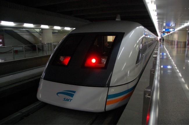
Just as with the growth of a bamboo plant, there are many situations that involve constant change over time. Consider, for example, the first commercial maglev train in the world, the Shanghai MagLev Train. It carries passengers comfortably for a 30-kilometer trip from the airport to the subway station in only eight minutes.[footnote]http://www.chinahighlights.com/shanghai/transportation/maglev-train.htm[/footnote] Suppose a maglev train were to travel a long distance, and that the train maintains a constant speed of 83 meters per second for a period of time once it is 250 meters from the station. How can we analyze the train’s distance from the station as a function of time? In this section, we will investigate a kind of function that is useful for this purpose, and use it to investigate real-world situations such as the train’s distance from the station at a given point in time. The function describing the train’s motion is a linear function, which is defined as a function with a constant rate of change, that is, a polynomial of degree 1. There are several ways to represent a linear function, including word form, function notation, tabular form, and graphical form. We will describe the train’s motion as a function using each method.
Another approach to representing linear functions is by using function notation. One example of function notation is an equation written in the form known as the slope-intercept form of a line, where [latex]x[/latex] is the input value, [latex]m[/latex] is the rate of change, and [latex]b[/latex] is the initial value of the dependent variable.
In the example of the train, we might use the notation [latex]D\left(t\right)[/latex] in which the total distance [latex]D[/latex] is a function of the time [latex]t[/latex]. The rate, [latex]m[/latex], is 83 meters per second. The initial value of the dependent variable [latex]b[/latex] is the original distance from the station, 250 meters. We can write a generalized equation to represent the motion of the train.
A third method of representing a linear function is through the use of a table. The relationship between the distance from the station and the time is represented in the table below. From the table, we can see that the distance changes by 83 meters for every 1 second increase in time.
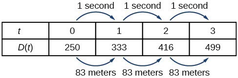
Tabular representation of the function D showing selected input and output values
Can the input in the previous example be any real number? No. The input represents time, so while nonnegative rational and irrational numbers are possible, negative real numbers are not possible for this example. The input consists of non-negative real numbers.
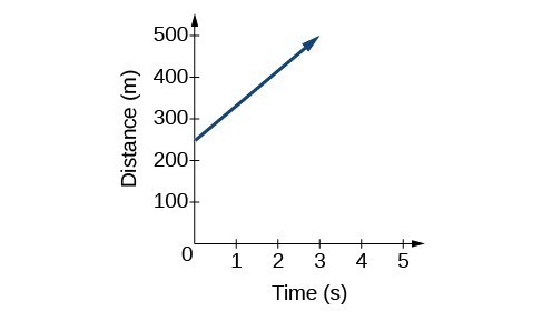
Another way to represent linear functions is visually, using a graph. We can use the function relationship from above, [latex]D\left(t\right)=83t+250[/latex], to draw a graph, represented in the graph below. Notice the graph is a line. When we plot a linear function, the graph is always a line. The rate of change, which is constant, determines the slant, or slope of the line. The point at which the input value is zero is the vertical intercept, or y-intercept, of the line. We can see from the graph that the y-intercept in the train example we just saw is [latex]\left(0,250\right)[/latex] and represents the distance of the train from the station when it began moving at a constant speed.
 A graph of an increasing function with points at (-2, -4) and (0, 2)." width="487" height="289" />
The graph of [latex]D\left(t\right)=83t+250[/latex]. Graphs of linear functions are lines because the rate of change is constant.
Notice that the graph of the train example is restricted, but this is not always the case. Consider the graph of the line [latex]f\left(x\right)=2
A linear function is a function whose graph is a line. Linear functions can be written in the slope-intercept form of a line
where [latex]b[/latex] is the initial or starting value of the function (when input, [latex]x=0[/latex]), and [latex]m[/latex] is the constant rate of change, or slope of the function. The y-intercept is at [latex]\left(0,b\right)[/latex].
The pressure, [latex]P[/latex], in pounds per square inch (PSI) on the diver in Figure 3 depends upon her depth below the water surface, [latex]d[/latex], in feet. This relationship may be modeled by the equation, [latex]P\left(d\right)=0.434d+14.696[/latex]. Restate this function in words.

(credit: Ilse Reijs and Jan-Noud Hutten)
Answer: To restate the function in words, we need to describe each part of the equation. The pressure as a function of depth equals four hundred thirty-four thousandths times depth plus fourteen and six hundred ninety-six thousandths.
The initial value, 14.696, is the pressure in PSI on the diver at a depth of 0 feet, which is the surface of the water. The rate of change, or slope, is 0.434 PSI per foot. This tells us that the pressure on the diver increases 0.434 PSI for each foot her depth increases.
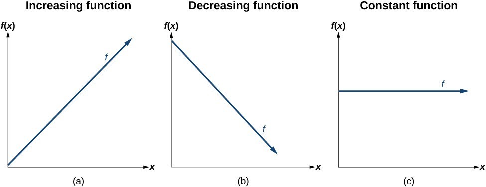
The linear functions we used in the two previous examples increased over time, but not every linear function does. A linear function may be increasing, decreasing, or constant. For an increasing function, as with the train example, the output values increase as the input values increase. The graph of an increasing function has a positive slope. A line with a positive slope slants upward from left to right as in (a). For a decreasing function, the slope is negative. The output values decrease as the input values increase. A line with a negative slope slants downward from left to right as in (b). If the function is constant, the output values are the same for all input values so the slope is zero. A line with a slope of zero is horizontal as in (c).
In the examples we have seen so far, we have had the slope provided for us. However, we often need to calculate the slope given input and output values. Given two values for the input, [latex]_[/latex] and [latex]_[/latex], and two corresponding values for the output, [latex]_[/latex] and [latex]_[/latex] —which can be represented by a set of points, [latex]\left(_\text_\right)[/latex] and [latex]\left(_\text_\right)[/latex]—we can calculate the slope [latex]m[/latex], as follows [latex-display]m=\frac>>=\frac=\frac<_-_><_-_>[/latex-display] where [latex]\Delta y[/latex] is the vertical displacement and [latex]\Delta x[/latex] is the horizontal displacement. Note in function notation two corresponding values for the output [latex]_[/latex] and [latex]_[/latex] for the function [latex]f[/latex], [latex]_=f\left(_\right)[/latex] and [latex]_=f\left(_\right)[/latex], so we could equivalently write [latex-display]m=\frac
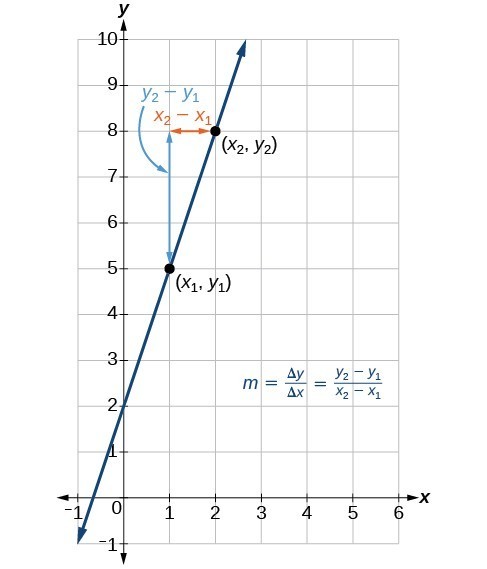
The slope of a function is calculated by the change in [latex]y[/latex] divided by the change in [latex]x[/latex]. It does not matter which coordinate is used as the [latex]\left(_>_\right)[/latex] and which is the [latex]\left(_,\text< >_\right)[/latex], as long as each calculation is started with the elements from the same coordinate pair.
Are the units for slope always [latex]\frac>>[/latex] ? Yes. Think of the units as the change of output value for each unit of change in input value. An example of slope could be miles per hour or dollars per day. Notice the units appear as a ratio of units for the output per units for the input.
The slope, or rate of change, of a function [latex]m[/latex] can be calculated according to the following: [latex-display]m=\frac>>=\frac=\frac_-_>_-_>[/latex-display] where [latex]_[/latex] and [latex]_[/latex] are input values, [latex]_[/latex] and [latex]_[/latex] are output values.
If [latex]f\left(x\right)[/latex] is a linear function, and [latex]\left(3,-2\right)[/latex] and [latex]\left(8,1\right)[/latex] are points on the line, find the slope. Is this function increasing or decreasing?
Answer: The coordinate pairs are [latex]\left(3,-2\right)[/latex] and [latex]\left(8,1\right)[/latex]. To find the rate of change, we divide the change in output by the change in input. [latex-display]m=\frac>>=\frac<1-\left(-2\right)>=\frac[/latex-display] We could also write the slope as [latex]m=0.6[/latex]. The function is increasing because [latex]m>0[/latex].
As noted earlier, the order in which we write the points does not matter when we compute the slope of the line as long as the first output value, or y-coordinate, used corresponds with the first input value, or x-coordinate, used.
If [latex]f\left(x\right)[/latex] is a linear function, and [latex]\left(2,3\right)[/latex] and [latex]\left(0,4\right)[/latex] are points on the line, find the slope. Is this function increasing or decreasing?
Answer: [latex-display]m=\frac=\frac=-\frac[/latex] ; decreasing because [latex]m<0[/latex-display]
The population of a city increased from 23,400 to 27,800 between 2008 and 2012. Find the change of population per year if we assume the change was constant from 2008 to 2012.
Answer: The rate of change relates the change in population to the change in time. The population increased by [latex]27,800-23,400=4400[/latex] people over the four-year time interval. To find the rate of change, divide the change in the number of people by the number of years. [latex-display]\frac>>=1,100\text< >\frac>>[/latex-display] So the population increased by 1,100 people per year.
Because we are told that the population increased, we would expect the slope to be positive. This positive slope we calculated is therefore reasonable.
The population of a small town increased from 1,442 to 1,868 between 2009 and 2012. Find the change of population per year if we assume the change was constant from 2009 to 2012.
| slope-intercept form of a line | [latex]f\left(x\right)=mx+b[/latex] |
| slope | [latex]m=\frac>>=\frac=\frac_-_>_-_>[/latex] |
| point-slope form of a line | [latex]y-_=m\left(x-_\right)[/latex] |
decreasing linear function a function with a negative slope: If [latex]f\left(x\right)=mx+b, \text